seqfam

Introduction

The seqfam package is primarily designed for analysing next generation sequencing (NGS) DNA data from families with known pedigree information in order to identify rare variants that are potentially causal of a disease/trait of interest. It uses the popular and versatile Pandas library, and can be straightforwardly integrated into existing analysis code/pipelines. Seqfam can be used to verify pedigree information, to perform Monte Carlo gene dropping, to undertake regression-based gene burden testing, and to identify variants which segregate by affection status in families via user-defined pattern of occurrence rules. Additionally, it can generate scripts for running analyses in a MapReduce pattern on a computer cluster, something which is usually desirable in NGS data analysis and indeed big data analysis in general.

Requirements and installation

Seqfam is compatible with Windows, Mac OX X and Linux operating systems. It is coded using Python 3.6 but can also be run by Python 2.7. It requires the following packages (listed in requirements.txt):

• pandas==0.20.3
• scipy==0.19.1
• natsort==5.1.1
• numpy==1.13.3
• setuptools==38.4.0
• statsmodels==0.8.0

Run the following commands to clone and install from GitHub.

$ git clone https://github.com/mframpton/seqfam
$ cd seqfam
$ pip install -r requirements.txt
$ python setup.py install

Tutorial

This section describes the functionality and methods employed by seqfam’s 5 modules, which are:

1. gene_drop: Monte Carlo gene dropping;
2. pof: variant pattern of occurrence in families;
3. gene_burden: regression-based gene burden testing;
4. relatedness: identification of duplicates and verification of ascertained pedigree information via kinship coefficients;
5. sge: Sun Grid Engine (SGE) array job creation.

Figure 1 provides a visual representation of modules 1–4.

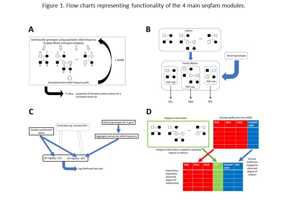
Panel A represents the Cohort.gene_drop() method in the gene_drop module which performs Monte Carlo gene dropping. On a single iteration, for each family the algorithm seeds founder genotypes based on the variant population allele frequency (AF) and then gene drops via depth-first traversals. Having done this for all families, a simulated cohort AF is calculated and following many iterations (e.g. 10,000), a p-value, the proportion of iterations where cohort AF < simulated cohort AF, is outputted. Panel B represents the Pof.get_family_pass_name_l() method in the pof module. Prior to calling the method, each family is assigned a variant pattern of occurrence (POF) rule. The method then takes a variant’s genotypes and returns families whose POF rule is passed. Panel C represents the CMC.do_multivariate_tests() method in the gene_burden module. This method takes sample affection status and variant genotypes across multiple genes, plus optionally covariates such as ancestry PCA coordinates. For each gene, the method aggregates the variants by AF, constructs h0 and h1 logit models which may include the covariates, and then performs a log-likelihood ratio test. Panel D represents the Relatedness.get_exp_obs_df() method in the relatedness module. For input, this takes pedigree information and kinship coefficients from KING for each within-family sample pair. It maps these data to expected and observed degrees of relationship respectively, returning a DataFrame.

The repository contains additional scripts in src/examples which demonstrate the functionality of the modules on example data, including files in the data directory. The scripts are 1_example_gene_drop.py, 2_example_pof.py, 3_example_gene_burden.py, 4_example_relatedness.py, and 5_example_sge.py. The reader can also refer to Table 1 for a summary of the main user functions of the 5 seqfam modules. Data in the example data files are derived from the whole exome sequencing of a large cohort of over 200 families with inflammatory bowel disease.

Table 1. Summary of main user functions in seqfam modules

Method	Description	Input	Output
gene_drop.Cohort.gene_drop()	Monte Carlo gene dropping	Cohort fam file (pedigree info), variant population AF, cohort AF, list of samples genotyped, # interactions	p-value
pof.Pof.get_family_pass_name_l()	Variant POF with respect to affected (& unaffected) members	Variant POF rule & genotypes	List of families whose POF rules is passed by variant
gene_burden.CMC.do_multivariate_tests()	Regression-based gene burden testing	Files containing samples, genotypes & covariates files; output path	Data frame and csv file containing burden test results
relatedness.Relatedness.find_duplicates()	Identify duplicates from kinship coefficient	KING sample pair kinship coefficient file	List of duplicates
relatedness.Relatedness.get_exp_obs_df()	Map pedigrees & kinship coefficients to expected & observed degrees of relationship	Cohort fam, KING within-family sample pair kinship coefficient file	Data frame of expected & observed degrees of relationship
sge.SGE.make_map_reduce_jobs()	Make computer cluster array job scripts.	Filename prefix, lists of map tasks, map tasks to execute and reduce tasks.	Scripts required to run array job including master submit script

gene_drop

For a rare variant to be considered potentially causal of a particular trait/disease based on in silico analysis, it should satisfy various criteria, such as being biologically plausible and predicted to be pathogenic. The gene_drop module can be used to further assess candidate variants via Monte Carlo gene dropping.

Given the structure of the families, Monte Carlo gene dropping can indicate whether a variant is enriched in the cohort relative to the general population, and assuming the trait/disease is more prevalent in the cohort, such enrichment supports causality. The gene_drop module can be considered complementary to the RVsharing R package [BYP+14] which calculates the probability of multiple affected relatives sharing a rare variant under the assumption of no disease association or linkage.

The module requires a pedigree file in fam format as input. The example script 1_example_gene_drop.py shows how to use gene_drop with the pedigrees in data/cohort.fam. It first creates a gene_drop.Cohort object from cohort.fam which stores all of the pedigrees as trees.

from seqfam.gene_drop import Cohort
...
cohort_fam = os.path.join(data_dir,"cohort.fam")
cohort = Cohort(cohort_fam)

For a hypothetical variant of interest, the script then specifies:

1. allele frequency in the general population (pop_af) is 0.025;
2. the subset of samples which have genotypes (sample_genotyped_l).

Now the gene dropping can be performed via the gene_drop.Cohort.gene_drop() method. The script uses the method to assess whether increasing cohort allele frequencies (cohort_af) indicate enrichment relative to the general population. For each cohort_af, the method returns an enrichment p-value (p), and so as cohort_af increases, p decreases.

pop_af = 0.025
for cohort_af in [0.025,0.03,0.035,0.04]:
       p = cohort.gene_drop(pop_af, cohort_af, sample_genotyped_l, 1000)

The method gene drops in a family in the following way. First, it assigns a genotype (number of copies of the mutant allele) to each founder using a Binomial distribution where the number of trials is 2 and the probability of success in each trial is pop_af. Hence the founders are assumed to be unrelated. It then performs a depth-first traversal starting from each founder (1 per spousal pair), and for heterozygotes, uses a random number generator to determine which parental allele to pass onto the child. Thus, every individual in the family is assigned a genotype.

By default, for each variant of interest, the method performs 10,000 iterations of gene dropping in the familial cohort. In each iteration it gene drops in each family once and then calculates the resulting simulated cohort allele frequency from the genotyped samples (sample_genotyped_l). After completing all iterations of gene dropping, the method returns the p-value (p), which is the proportion of iterations where cohort_af is less than or equal to the simulated cohort allele frequency. A low proportion, e.g. < 5%, can be taken as evidence of enrichment.

pof

Like gene_drop, the pof module can provide additional evidence for whether particular rare variants are causal of a particular trait/disease. It is intended for identifying variants which are carried by most or all affected members of a family (As), or even which segregate between As and unaffected members (Ns).

For each family, the user uses the pof module to define a variant pattern of occurrence (POF) rule and check whether any supplied variants pass. The rule can specify a minimum value for the proportion As who are carriers (A_carrier_p), and/or a minimum difference between the proportion of As and Ns who are carriers (AN_carrier_diff). Constraints for the number of genotyped As and Ns can also be added, (A_n_min and N_n_min respectively).

The example script 2_example_pof.py provides an illustrative example. It first creates a couple of pof.Family objects to represent 2 families and their POF rule.

import pandas as pd
from seqfam.pof import Family,Pof

...

family_1 = Family("1","A3N2",["1_1","1_2","1_3"],["1_4","1_5"],A_n_min=3,N_n_min=2,AN_carrier_diff=0.5)
family_2 = Family("2","A4N1",["2_10","2_11","2_12","2_13","2_14"],["2_15"],A_n_min=4,N_n_min=1,A_carrier_p=1.0)

Family 1 is specified as having 3 As and 2 Ns, and its POF rule requires AN_carrier_diff to be 0.5. Family 2 has 4 As and 1 N, and a rule requiring all the As to be carriers. The rule in both families requires all members to be genotyped (see the A_n_min and N_n_min parameters).

The script next makes the genotypes for a hypothetical variant in a Pandas Series called variant_genotypes_s. Finally, it creates a pof.Pof object from the 2 pof.Family objects, and then calls the pof.Pof.get_family_pass_name_l() method to obtain a list of the families whose POF rule is passed by this variant.

family_l = [family_1,family_2]
pof = Pof(family_l)
family_pass_l = pof.get_family_pass_name_l(variant_genotypes_s)
print(family_pass_l)

gene_burden

The gene_burden.py module implements the Combined Multivariate and Collapsing (CMC) burden test [LL08] for detecting rare causal variants, where the multivariate test is a log-likelihood ratio test. The user can supply covariates to control for potential confounders such as divergent ancestry. This burden test should be applied to unrelated samples, and hence is of no use for cohorts containing few families. However, for cohorts containing a relatively large number of families, a sufficient number of unrelated cases can be extracted and pooled with a separate set of unrelated controls. Burden tests aggregate rare variants in a gene or functional unit into a single score ([LL08]; [MR09]; [ME10]; [PKdB+10], and are one broad class of statistical methods which combine the effects of rare variants in order to increase power over single marker approaches. Sequence kernel association testing (SKAT) [WLCeal11] is another widely-used sub-category of such methods. In general, burden testing is more powerful than SKAT when a large proportion of variants are causal and are all deleterious/protective.

The 3_example_gene_burden.py script shows how to use the gene_burden module to perform CMC tests which control for covariates. Here, we say that variants are grouped by the tested units (gene / other functional unit), and within the groups, they are aggregated, usually within population allele frequency (PAF) ranges. Aggregation means that within each aggregation category (e.g. PAF < 1%), an individual sample is given the value 1 if it carries any variants, otherwise 0. The example script performs 1 CMC test per gene (i.e. it groups variants by gene), where variants are aggregated within 2 PAF ranges: PAF \(<\) 1% and 1% \(\leq\) PAF \(<\) 5% (any variants with PAF \(\geq\) 5% remain unaggregated).

The input files are in the data/gene_burden directory: samples.csv, genotypes.csv and covariates.csv. The samples.csv file contains the samples’ ID and affection status where 2 indicates a case and 1 a control. The genotypes.csv file can be created by combining genotypes from a VCF file with variant annotations (e.g. from the Variant Effect Predictor). It contains 1 row per variant with columns for the sample genotypes (the number of alternate alleles), plus columns for variant grouping and aggregation e.g. gene and PAF. The covariates.csv file contains the covariates to control for, which in this instance are ancestry Principal Components Analysis (PCA) coordinates.

The script first reads samples.csv into a Pandas Series, and genotypes.csv and covariates.csv into Pandas DataFrames. These DataFrames are indexed by variant ID and covariate name respectively.

import pandas as pd
from seqfam.gene_burden import CMC
...
#Read the samples into a Series.
sample_s = pd.read_csv(samples_path, dtype=str, index_col="Sample ID")
sample_s["Affection"] = sample_s["Affection"].astype(int)
sample_s = sample_s[sample_s != 0]

#Read the variant annotations + genotypes into a DataFrame.
variant_col,gene_col = "VARIANT_ID","Gene"
pop_frq_col_l = ["database1_AF","database2_AF","database3_AF"]
geno_df = pd.read_csv(genotypes_path, dtype=str, usecols=[variant_col,gene_col] + pop_frq_col_l + sample_s.index.tolist(), index_col=variant_col)
geno_df.loc[:,pop_frq_col_l] = geno_df.loc[:,pop_frq_col_l].apply(pd.to_numeric, axis=1)
geno_df.loc[:,sample_s.index] = geno_df.loc[:,sample_s.index].apply(pd.to_numeric, errors='coerce', downcast='integer', axis=1)
geno_df.loc[:,sample_s.index] = geno_df.loc[:,sample_s.index].fillna(0)

#Read the covariates into a DataFrame.
covar_df = None if covariates_path == None else pd.read_csv(covariates_path, index_col=0)

Having created a gene_burden.CMC object, the script calls its gene_burden.CMC.assign_variants_to_pop_frq_cats() method in order to map the variants to the desired PAF range categories. Multiple PAF columns (databases) are used here, ordered by descending preference. The mapping is stored in a new pop_frq_cat column in the genotypes DataFrame.

cmc = CMC()
geno_df = cmc.assign_variants_to_pop_frq_cats(geno_df, pop_frq_col_l, {"rare":0.01,"mod_rare":0.05})

Finally, the script calls the gene_burden.CMC.do_multivariate_tests() method to perform the CMC tests, specifying the gene column for grouping the variants, and the new pop_frq_cat column for aggregation.

agg_col = "pop_frq_cat"
cmc_result_df = cmc.do_multivariate_tests(sample_s, geno_df, group_col=gene_col, agg_col="pop_frq_cat", agg_val_l=["rare","mod_rare"], covar_df=covar_df, results_path=results_path)

For each gene, this method performs a multivariate test, which is a log-likelihood ratio test based on Wilk’s theorem:

\[\chi^2 = 2(ll_{h0} - ll_{h1}); df = df_{h1} - df_{h0}\]

where ll is log-likelihood, h1 is the alternative hypothesis, h0 is the null hypothesis and df is degrees of freedom. Specifically, it is a log-likelihood ratio test on null and alternative hypothesis logit models where the dependent variable is derived from affection status, the variant variables (aggregated and/or unaggregated) are independent variables in the alternative model and the covariates are independent variables in both. The logit models are fitted using the Broyden–Fletcher–Goldfarb–Shanno (BFGS) algorithm.

The results are written to a CSV (comma-separated values) file (results_path) and also returned in a DataFrame (cmc_result_df). They include the number of variants in each aggregation category (rare, mod_rare), the number of unaggregated variants (unagg), the proportion of affecteds and unaffecteds which have value 1 for each variant variable (rare_aff_p … unagg_unaff_p), the log-likelihood ratio test p-value with/without covariates (llr_p and llr_cov_p), and the coefficient/p-value for each aggregated variant variable and covariate in the h1 logit model (rare_c, rare_p … PC5_c, PC5_p).

>>> print(cmc_result_df.head().to_string())
         rare  mod_rare  unagg  rare_aff_p  rare_unaff_p  mod_rare_aff_p  mod_rare_unaff_p  unagg_aff_p  unagg_unaff_p         llr_p  llr_cov_p     rare_c    rare_p  mod_rare_c  mod_rare_p     PC1_c         PC1_p     PC2_c         PC2_p     PC3_c         PC3_p     PC4_c         PC4_p     PC5_c     PC5_p
Gene
GENE_81    17         4      0    0.083333      0.041667        0.340909          0.090909          NaN            NaN  8.776693e-11   0.000075   0.260649  0.607068    1.317017    0.000041  0.350426  2.719782e-10  0.742543  9.178604e-11 -0.286762  1.989026e-10 -0.933229  2.921982e-26 -0.196124  0.100419
GENE_10     1         0      0    0.000000      0.003788             NaN               NaN          NaN            NaN           NaN   0.009316 -11.325180  0.825768         NaN         NaN  0.347303  3.341802e-10  0.670772  1.993786e-09 -0.289419  9.064199e-11 -0.978531  2.720945e-28 -0.193831  0.096250
GENE_16     4         0      0    0.007576      0.034091             NaN               NaN          NaN            NaN           NaN   0.013386  -2.475089  0.014941         NaN         NaN  0.337994  7.855867e-10  0.698458  4.950072e-10 -0.282116  2.037413e-10 -0.972062  6.228652e-28 -0.154929  0.185172
GENE_59     3         0      0    0.000000      0.011364             NaN               NaN          NaN            NaN           NaN   0.014363 -10.955116  0.897996         NaN         NaN  0.333042  1.325734e-09  0.675311  1.539985e-09 -0.284952  1.417334e-10 -0.961612  3.308430e-28 -0.176737  0.128946
GENE_15     2         0      0    0.000000      0.007576             NaN               NaN          NaN            NaN           NaN   0.027556 -10.728126  0.894869         NaN         NaN  0.329435  1.331849e-09  0.697045  6.262195e-10 -0.281625  2.635041e-10 -0.956502  6.064632e-28 -0.185669  0.109201

If the user ran the tests without covariates, then the returned results DataFrame would not include the llr_cov_p and PC covariate columns, and the columns rare_c … mod_rare_p would correspond to the coefficient/p-value in the h0 logit model.

relatedness

The potential for genetic discovery in DNA sequencing data is reduced when samples are mislabelled. Hence, necessary quality control steps include identifying duplicates, and in the case of familial samples, verifying the ascertained familial relationships described in the pedigrees. The relatedness module facilitates these quality control steps and is used in conjunction with KING software [MMReal10]. Given genotypes for relatively common variants, KING can efficiently calculate a kinship coefficient for each sample pair. The relatedness module can then map each kinship coefficient to a degree of relationship and check it corresponds with the pedigree. KING is often already part of NGS analysis pipelines, so incorporating relatedness is straightforward. Peddy [PQ17] is an alternative which does not require KING.

As input, the relatedness module requires a pedigree information file in fam format and a kinship coefficients file from KING, either containing within or between-family sample pairs. The example script 4_example_relatedness.py uses data/cohort.fam for the former and data/relatedness/king.kinship.ibs (within-family sample pairs) for the latter. It creates a relatedness.Relatedness object with these paths, and then calls the object’s relatedness.Relatedness.find_duplicates() and relatedness.Relatedness.get_exp_obs_df() methods.

from seqfam.relatedness import Relatedness
import pandas as pd
...
relatedness = Relatedness(wf_file=wf_file,cohort_tsv=cohort_tsv,bf_file=None)

#Within-family duplicates.
wf_duplicate_l = relatedness.find_duplicates(bf_b=False)
print(wf_duplicate_l)
#Between-family duplicates... (Uncomment if you have a bf_file).
#bf_duplicate_l = relatedness.find_duplicates(bf_b=True)
#print(bf_duplicate_l)

#Expected versus observed within-family relationships.
exp_obs_df = relatedness.get_exp_obs_df()

The relatedness.Relatedness.find_duplicates() method returns a list of any duplicate samples, and the relatedness.Relatedness.get_exp_obs_df() method returns a Pandas DataFrame containing the expected and observed degree of relationship for each within-family sample pair.

>>> print(wf_duplicate_l)
['171b_1448,171b_1449']
>>> print(exp_obs_df)
                 EXP_REL  Kinship OBS_REL
FAMILY ID1  ID2
1      44   47         1   0.2584       1
2      6    20         4   0.0390       4
            21         4   0.0688       3
       20   21         4   0.0051       4
3      501  838        1   0.2052       1
            844        2   0.1081       2
       838  844        1   0.2572       1
...

The user can modify the mapping from kinship coefficient to relationship degree, but by default it is as specified in KING documentation: > 0.354 for duplicate samples/monozygotic twins, 0.177–0.354 for 1st degree relatives, 0.0884–0.177 for 2nd degree relatives, 0.0442–0.0884 for 3rd degree relatives, and < 0.0442 for unrelated. The final line of the script prints the sample pairs which have a different expected and observed degree of relationship.

print(exp_obs_df.loc[(exp_obs_df["EXP_REL"]!=exp_obs_df["OBS_REL"]) & (pd.notnull(exp_obs_df["Kinship"])),:])

sge

The sge module has general utility in analysing NGS data, and indeed any big data on computer clusters. Many NGS data analyses can be cast as “embarassingly parallel problems” and hence executed more efficiently on a computer cluster via a MapReduce pattern: the overall task is decomposed into independent sub-tasks (map tasks) which run in parallel, and on their completion, a reduce action merges/filters/summarises the results. For example, gene burden testing across the whole exome can be decomposed into independent sub-tasks by splitting the exome into sub-units e.g. chromosomes. Sun Grid Engine (SGE) is a widely used batch-queueing system, and analyses can be performed in a MapReduce pattern on SGE via array jobs. Given a list of map tasks and the reduce task(s), the sge module can create the scripts for submitting and running an array job.

The script 5_example_sge.py provides an example. It first makes lists of map tasks (map_task_l) and map tasks to execute (map_task_exec_l) via the custom get_map_task_l function (see the script), and then a reduce task string (reduce_tasks). While map_task_l contains all map tasks, map_task_exec_l contains the subset which have not yet completed successfully and hence need to run.

from seqfam.sge import SGE
...
print("Making map and reduce tasks...")
chr_l = [str(chrom) for chrom in range(1,23)] + ["X","Y"]
[map_task_l, map_task_exec_l] = get_map_task_l(chr_l)
reduce_tasks = "\n".join(["python 2_merge_results.py","python 3_summarise_results.py"])

Next, the script creates an sge.SGE object which stores the directory where job scripts will be written (the variable script_dir which here has the value data/sge). Finally it calls the object’s sge.SGE.make_map_reduce_jobs() method with the following arguments: a job script name prefix (here test), map_task_l, map_task_exec_l and reduce_tasks.

sge = SGE(script_dir)
sge.make_map_reduce_jobs("test", map_task_l, reduce_tasks, map_task_exec_l)

This writes the job scripts, and were they for a real array job (they are not), the user could submit it to the job scheduler by running the master executable submit script submit_map_reduce.sh. The generated file test.map_task_exec.txt specifies which map tasks to run (map_tasks_exec_l).

References

[BYP+14]

A. Bureau, S. G. Younkin, M. M. Parker, J. E. Bailey-Wilson, M. L. Marazita, J. C. Murray, E. Mangold, H. Albacha-Hejazi, T. H. Beaty, and I. Ruczinski. Inferring rare disease risk variants based on exact probabilities of sharing by multiple affected relatives. Bioinformatics, 30(15):2189–2196, Aug 2014.

[LL08]

(1, 2) B. Li and S. M. Leal. Methods for detecting associations with rare variants for common diseases: application to analysis of sequence data. Am. J. Hum. Genet., 83(3):311–321, Sep 2008.

[MR09]

B. E. Madsen and Browning S. R. A groupwise association test for rare mutations using a weighted sum statistic. PLoS Genetics, 2009.

[MMReal10]

A. Manichaikul, J. C. Mychaleckyj, S. S. Rich, and et al. Robust relationship inference in genome-wide association studies. Bioinformatics, 26(22):2867–2873, 2010.

[ME10]

A. P. Morris and Zeggini E. An evaluation of statistical approaches to rare variant analysis in genetic association studies. Genetic Epidemiology, 34(2):188–193, 2010.

[PQ17]

B. S. Pedersen and A. R. Quinlan. Who’s Who? Detecting and Resolving Sample Anomalies in Human DNA Sequencing Studies with Peddy. Am. J. Hum. Genet., 100(3):406–413, Mar 2017.

[PKdB+10]

A. L. Price, G. V. Kryukov, P. I. de Bakker, S. M. Purcell, J. Staples, L. J. Wei, and S. R. Sunyaev. Pooled association tests for rare variants in exon-resequencing studies. Am. J. Hum. Genet., 86(6):832–838, Jun 2010.

[WLCeal11]

M. C. Wu, S. Lee, T. Cai, and et al. Rare-variant association testing for sequencing data with the sequence kernel association test. American Journal of Human Genetics, 89(1):82–93, 2011.

API reference

gene_drop

class gene_drop.Cohort(cohort_fam)

Represents a cohort of familial individuals as a list of FamilyTree objects.

gene_drop(pop_af, cohort_af, sample_genotyped_l, gene_drop_n)

Perform gene dropping across the cohort and return the proportion of iterations in which the simulated allele frequency is less than or equal to the cohort frequency.

Args:

pop_af (float): population allele frequency.

cohort_af (float): cohort allele frequency.

sample_genotyped (list of strs): the list of samples genotyped for this variant from which cohort af was calculated.

gene_drop_n (int): number of iterations to perform.

Returns:

cohort_enriched_p (float): proportion of iterations in which the simulated allele frequency is less than or equal to the cohort frequency.

get_all_family_l()

Get a list of all the families in the cohort.

Returns:

all_family_l (list): list of IDs of families present in cohort.

get_all_sample_l()

Get a list of all of the samples in the cohort.

Returns:

all_sample_l (list): list of sample IDs tuples (<FAMILY_ID>,<INDIVIDUAL_ID>).

make_fam_tree(ped_df)

For a family, make a list of Nodes and from these, a Family Tree.

Args:

ped_df (pandas.core.frame.DataFrame): contains the pedigree information for the family.

Returns:

family_tree (FamilyTree obj): represents the family.

remove(family_l)

Remove families from the cohort (self.fam_tree_l).

class gene_drop.FamilyTree(logger, id, node_l)

Represents a family tree with node objects and has methods to perform gene-dropping.

gene_drop(pop_af, ind_gtyped_l)

Main method for performing gene dropping for 1 variant in this family tree.

Args:

pop_af (float): population allele frequency of the variant.

ind_gtyped_l (list of strs): IDs of individuals in this family who have a genotype for the variant.

Returns:

carrier_allele_count (int): the number of (genotyped) carriers in the family after dropping the gene.

gene_drop_dfs(start_node)

Perform gene dropping in the family tree starting from the specified start node and using a depth-first traversal.

Args:

start_node (Node): node from which to start the gene dropping.

Returns:

visited (set): nodes visited during the depth-first traversal.

log_all_genotypes()

Log all of the node genotypes.

log_all_info()

Log all of the information about each node in the family tree.

set_offspring_genotype(node)

Set a node’s genoytpe based on its parents’ genotypes. If the parent is heterozygous then the probability of the variant allele being passed to the offspring is 0.5.

Args:

node (Node): the node whose genotype will be set.

class gene_drop.Node(id, parent_l, spouse, children_l)

Represents an individual (node) in a family tree.

get_summary_str()

Get a summary string for the node.

Returns:

summary_str: the object attributes as a string.

class gene_drop.NodeGenerator

Generates nodes to represent individuals in a pedigree.

convert_ped_df_to_node_l(ped_df)

Create the nodes.

Args:

ped_df (DataFrame):

Returns:

node_l (list of Nodes): the Node objects represent the individuals in the pedigree DataFrame.

set_relationships(ped_row_s, name_node_dict)

Set the relationships between the nodes.

Args:

ped_row_s (Series): row from a pedigree dataframe, representing 1 individual.

name_node_dict (dictionary): maps from node name to node.

gene_burden

class gene_burden.CMC

Implements the combined multivariate and collapsing (CMC) burden test, where the multivariate test is a log-likelihood ratio test.

aggregate_by_agg_col(geno_df)

Aggregate genotypes within variant population frequency categories.

Args:

geno_df (DataFrame): index is the variant ID and columns must include (1) group_col (see below); (2) agg_col (see below); (3) sample genotypes (# copies of alternate allele 0-2).

Returns:

geno_agg_df (DataFrame): index is the gene & variant aggregation category, and columns are the # of variants for each sample.

assign_variants_to_pop_frq_cats(geno_df, pop_frq_col_l, pop_frq_cat_dict)

Assign variants to allele population frequency range categories.

Args:

geno_df (DataFrame): index is the variant ID and columns must include the population allele frequency columns listed in the pop_frq_col_l parameter (see below)

pop_frq_col_l (list of str): contains the names of the population allele frequency columns in descending order of preference.

pop_frq_cat_dict (dict of (str,float)): mapping of frequency category name to exclusive upper bound.

Returns:

geno_df (DataFrame): the inputted geno_df DataFrame with an extra column for the variant aggregation category (“pop_frq_cat”).

do_multivariate_test(geno_agg_gene_df, y, covar_df=None)

Do a multivariate test for 1 gene.

Args:

geno_agg_gene_df (DataFrame): index is the gene & variant aggregation category, and columns are the # of variants for each sample.

y (numpy.ndarray): values are 0/1 (unaffected/affected).

covar_df (DataFrame): index is the covariate names and columns are samples.

Returns:

test_result_s (Series): multivariate test results for 1 gene/functional unit containing (1) llr_p (and llr_cov_p), the log-likelihood ratio p-value (after controlling for covariates); (2) coefficient & p-value for each independent variable.

do_multivariate_tests(sample_s, geno_df, group_col, agg_col, agg_cat_l, covar_df=None, results_path=None)

Main method for doing multivariate tests.

Args:

sample_s (Series): index is the sample names, and values are 1/2 (unaffected/affected).

geno_df (DataFrame): index is the variant ID and columns must include (1) group_col (see below); (2) agg_col (see below); (3) sample genotypes (# copies of alternate allele 0-2).

group_col (str): column in geno_df identifying the groups of variants to be tested for association with the phenotype e.g. gene, pathway or any other entity.

agg_col (str): column containing the aggregation categories (e.g. population allele frequency range) - variants in the same group and aggregation category will be aggregated (collapsed into a dichotomous variable 0/1).

agg_cat_l (list of strs): specifies which aggregation categories to present results for (i.e. coefficient and p-value in the alternative hypothesis logit model).

covar_df (DataFrame): index is the covariate names and columns are the samples.

results_path (str): path to results file.

Returns:

result_df (DataFrame): multivariate test results, where the index is the variant group (e.g. gene) and columns are (1) # variants in each aggregated (& unaggregated) category; (2) proportion of (un)affecteds carrying a variant in each aggregated (& unaggregated) category; (3) llr_p (and llr_cov_p), the log-likelihood ratio p-value (after controlling for covariates); (4) coefficient & p-value for each independent variable.

fit_logit_model(X_df, y)

Fit a logit model.

Args:

X_df: the independent variables (covariates and or aggregated genotypes) for 1 gene.

y (numpy.ndarray): values are 0/1 (unaffected/affected).

Returns:

logit_result (statsmodels.discrete.discrete_model.BinaryResultsWrapper): contains results from fitting logit regression model.

get_agg_cat_count_df(geno_agg_df)

For each group in group_col (e.g. gene), get the number of variants in each variant aggregation category (in agg_col) e.g. population allele frequency range.

Args:

geno_agg_df (DataFrame): index is the gene & variant aggregation category, and columns are the # of variants for each sample.

Returns:

agg_cat_count_df (DataFrame): index is the gene and columns are # variants in each aggregated category and # unaggregated.

get_agg_cat_prop_by_affection(geno_agg_df)

For each group in group_col (e.g. gene), get the proportion of (un)affecteds who are carriers in each variant aggregation category (in agg_col) e.g. population allele frequency range.

Args:

geno_agg_df (DataFrame): index is the group_col & aggregation category, and columns are the # of variants for each sample.

Returns:

agg_cat_prop_df(DataFrame): index is the group_col, and columns indicate the proportion of (un)affected carriers in each variant aggregation category, plus unaggregated variants.

get_coef_pval_l(logit_result, covar_b=False)

Get the coefficients and corresponding p-values of the independent variables in the logit model.

Args:

logit_result (statsmodels.discrete.discrete_model.BinaryResultsWrapper): contains results from fitting logit regression model.

Returns:

coef_pval_l (list): list of coefficients and corresponding p-values.

pof

class pof.Family(name, category, A_l, N_l, A_n_min=0, N_n_min=0, A_p_min=None, AN_p_diff_min=None)

Represents a Family with various attributes: name, category (with respect to number of affected and unaffected members), IDs of affected and unaffected members, plus attributes relating to conditions which must be satisfied for a variant to “pass” in the family. These are the minimum number of affected members who are carriers, the minimum number of unaffecteds who are carriers, the minimum proportion of affecteds who are carriers, and the minimum difference in the proportion of affecteds and unaffecteds who are carriers.

log_info()

Log the object attributes.

pass_po(variant_genotypes_s, no_call='NA', carrier_call=['1', '2'])

Check whether a variant passes in the family.

Args:

variant_genotypes_s (Series): the genotypes of family members for the variant of interest.

no_call (str): how a no-call is represented in the genotype data.

carrier_call (list of strs): genotypes which correspond to carrying the variant.

Returns:

boolean: whether the variant passes.

class pof.Pof(family_l)

Pattern of (variant) occurrence: stores a list of family objects, and has a function to check if the genotypes for a variant of interest satisfy the sepcified pattern of occurence criteria in any of these families.

get_family_pass_name_l(variant_genotypes_s)

Checks whether the genotypes for a variant of interest satisfy the specified pattern of occurrence criteria (pass) in any of the supplied families.

Args:

variant_genotypes_s (Series): contains the genotypes for the variant of interest for all individuals in the families contained in the family_l attribute.

Returns:

pass_l (list of Family objects): the list of families in which the variant of interest passes.

relatedness

class relatedness.Relatedness(bf_file=None, wf_file=None, cohort_fam=None, kinship_coef_thresh_dict={'0': 0.354, '1': 0.177, '2': 0.0844, '3': 0.0442})

Provides methods to find duplicates either between or within families, and to identify pairs of individuals within a family whose observed relationship (KING kinship coefficient) is different than expected given the pedigree.

convert_tuple_to_ids(duplicate_pair_tuple)

Convert a tuple containing the IDs of 2 duplicate individuals into a string.

Args:

duplicate_pair_tuple (tuple): tuple containing IDs of 2 duplicate individuals.

Returns:

duplicate_pair_str (str): string containing IDs of the 2 duplicate individuals.

find_duplicates(bf_b=True)

Find either between-family or within-family duplicates using the corresponding KING kinship coefficient output.

Args:

bf_b (boolean): whether to look for duplicates from different families (True) or duplicates within the same family, defaults to True.

Returns:

duplicate_l (list of strs): pairs of identified duplicates.

get_exp_obs_df()

Make a DataFrame containing the expected and observed relationships for individuals in the same family.

Returns:

exp_obs_df (DataFrame): contains columns for the expected and observed relationships.

get_exp_rel(ind_pair_s, relations_df)

Get the expected degree of relationship (1-4) between a pair of individuals.

Args:

ind_pair_s (Series): the IDs of a pair of individuals.

Returns:

exp_rel (str): the expected degree of relationship.

get_exp_rel_df(fam_df, fam_ind_seq_dict)

Make a dataframe containing the expected relationships between individuals in a family.

Args:

fam_df (DataFrame): contains the pedigree information for a family.

Returns:

exp_rel_df (DataFrame): contains the expected relationships between the family members.

get_kinship_coef(s)

Retrieve the kinship coefficient from a Series representing a row in a KING output file.

Args:

s (Series): represents a row in a KING output file.

Returns:

kinship_coef (str): kinship coefficient in the row.

get_relations_s(ind, fam_df)

For 1 individual, get a series containing lists of their siblings, parents and grandparents.

Args:

ind (str): individual ID

fam_df (DataFrame): contains the pedigree information for a family.

Returns:

relations_s (Series): contains lists of the individual’s siblings, parents, grandparents and great-grandparents.

sge

class sge.SGE(scripts_dir)

This class can create the scripts required for submitting and running an array job on a computer cluster with a Sungrid Engine job scheduler.

make_map_reduce_jobs(prep, map_task_l, reduce_task, map_task_exec_l=[], mem='14G')

Delete existing .sh files in the scripts dir.

misc

class misc.Logger

Class for time-stamped logging.

log(txt)

Prints a time-stamped text string.

Args:

txt (str): text string to print.